Reflection and Refraction

January 25,2016

On this day we conducted an experiment on reflection and refraction.

The conducted experiment had three objectives. Using an optical disk, we were to investigate the reflection and refraction of light. Another objective was the measurement of the index of refraction of a material using the optics set-up. Lastly, we were to trace the path of light as it emerges from optical materials of different geometries.

We were supposed to do an experiment on thermodynamics instead of this experiment.

I love light. It amuses me. I was excited to do the experiment because it dealt with the properties of light.

Before we started doing the experiment, we first borrowed the materials that were to be used.

The first part of the experiment was the alignment of the optics. Basically, the light source and the optical disk were mounted on the optical bench with the slit plate and slit mask in between them, respectively. A single ray coincident on the zero degrees-zero degrees axis of the optical disk was to be produced with the set-up orientation. This part was not very hard at all.

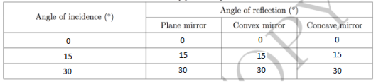
The second part of the experiment was to do the reflection by plane and spherical mirrors. The plane mirror was placed on the disk such that the mirror coincides with the 90 degrees-90 degrees axis of the optical disk. It was made sure that the center of the mirror and the center of the optical disk coincided. The optical disk was rotated such that the light would hit the plane mirror at 0,15 and 30 degrees. The angles at which the light was reflected were recorded. The same procedure was done for the convex and concave mirrors. Table 1 below shows the obtained angles. It can be seen that the angle of reflection is the same as the angle of incidence when light is to be focused on a mirror.
Table 1. Refraction by plane and spherical mirrors

The second part of the experiment dealt mainly with the refraction in glass. The mirror was replaced with a cylindrical lens. The flat surface of the glass coincided with the component axis of the optical disk. The alignment of the centers was made sure. The optical disk was rotated 5 times such that the light would hit the semicircular glass at 10,20,30,40 and 50 degrees. The index of refraction of the glass was calculated using Snell’s law.

Figure 1. Snell’s Law. Picture obtained from : 12physics.blogspot.com

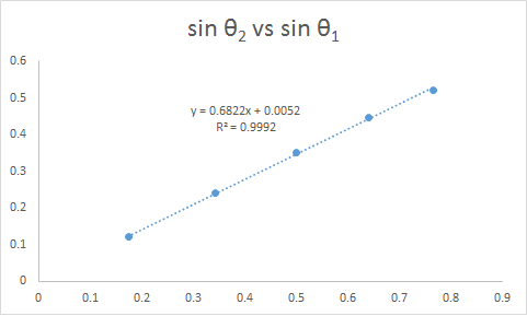
Figure 2. Relationship of the sines of the angles of incidence and refraction when incident ray strikes flat surface

 

By looking at the trend line in Figure 2, it can be seen that the slope is 0.6822. This means that the ratio of the indices of refraction of gas and the glass is 0.6822. Further calculations using Snell’s law would give us the index of refraction of the glass which is 1.47.

The next part of the experiment was to rotate the optical disk ( not the semicircular glass) by 180 degrees such that the incident ray strikes the curved side of the glass. It was made sure that the incident ray would strike the curved surface and pass through the center of the disk and the center of the flat surface for the reflected and refracted ray to coincide with the 0 degrees-0 degrees axis. The difference of this set-up with the previous one is that which medium comes first. In this set-up, the incident ray strikes the curved surface. In the previous set-up, the incident ray strikes the flat surface.

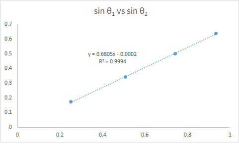
Figure 3. Relationship of the sines of the angles of incidence and refraction when incident ray strikes curved surface.

Based on Figure 3 and with the corresponding calculations using Snell’s law, the obtained index of refraction is still 1.47. This means that regardless whether the curved surface is struck first or not, the index of refraction would not change because it is a property of the glass. What would change is the angle of refraction.

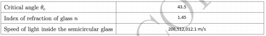
The last part dealt with total internal reflection. The set-up from the previous part was still used. The optical disk was rotated and the angle at which the refracted ray is parallel to the flat surface was to be found. It can be seen in Table 2 that the critical angle was found to be 43.5 degrees. The index refraction the glass can be obtained by plugging in the critical angle as θ1 and 90 degrees as θ2. The speed of light inside the semicircular glass was calculated using definition of the index of refraction : the ratio of the speed of light in vacuum and speed of light in a medium.

Table 2. Total internal reflection

Overall, the experiment was fun and easy. I hope the experiments to come will be easy and fun as well.

Woo! Achievement unlocked! First blog ever! First blog post ever!

Gas Laws

Last April 11, we conducted an experiment to verify two gas laws : Boyle’s and Charles’ Laws.

The ideal gas model is used to describe the behavior of dilute gases at low pressures and high temperatures. The ideal gas model is described by the Boyle’s Law, Charles’ Law, and Gay-Lussac’s Law. However, for this experiment Gay-Lussac’s Law will not be done.

So here’s a little background on the Boyle’s and Charles’ Laws.

Back in 1662, a guy named Robert Boyle discovered that at about one atmospheric pressure and at temperatures close to room temperature, the pressure and volume of gases are inversely proportional to each other and this relationship became known as Boyle’s Law. Boyle’s Law can be written mathematically as [1]

Equation (1)

where V is the volume of the gas, Cb is the proportionality constant which is equal to NkT, and P is the pressure. N is the number number of particles, k is the Boltzmann constant, and T is the temperature in Kelvin.

So the first thing we did was to set-up the experiment. First, a beaker was filled with water up to 3/4 full and the water was boiled. The water was boiled throughout the activity. The air chamber can was then connected to the mass lifter apparatus using the rubber tubing. The air chamber can was then placed in the hot bath. The piston was lifted to its maximum height and the gas pressure sensor was connected to the Vernier LabQuest. The temperature T was monitored throughout the experiment. A 50 g standard mass was placed on the platform of the mass lifter apparatus and the height h  of the piston and the pressure P was recorded. The previous step was also done for the 100,150,200 and 250 g masses.

The volume of the cylinder Vcyl for each height was computed. The reciprocal P-1 of each pressure reading was computed. A plot of Vcyl vs P-1 was done. The number of particles N and the volume of the air chamber can Vcham were calculated from the slope and y-intercept, respectively.

The measured diameter of the piston was 0.0325m. Table 1 below shows us that as we increase the mass of the object that we place, the height decreases and the pressure increases as well.

Table 1 .Experimental Data from the Boyle’s Law Experiment

Figure 1. Vcyl versus 1/P graph

The information that we got from the linear fit equation are the following :

The second part of the experiment was to conduct the Charles’ Law experiment. Back in 1780,  Jacques Charles discovered that at temperature close to room temperature and pressure about one atmospheric pressure, the volume and temperature of gases are directly proportional to each other. This can be mathematically represented as [1]

Equation (2)

where Cc is the proportionality constant which is equal to Nk/P.

The first step in this part of the experiment was to remove the beaker  (will serve as the hot bath) from the top of the stove. The air chamber was placed in the hot bath. The pressure P was monitored throughout the experiment. The temperature T of the hot bath was measured using a digital thermometer and the initial height h of the piston was recorded. Chunks of ice were slowly added on the hot bath while taking h and T measurements at equal time intervals. A V vs T plot was made. The number of particles N and the volume of the air chamber can Vcham were calculated from the slope and y-intercept, respectively.

Table 2. Experimental Data from the Charles’ Law Experiment

The data from table 2 tells us that as the temperature decreased, the height decreased which means that the volume decreased.

From the equation of the linear fit of the graph, we obtained the following data:

The experiment was a success in verifying Boyle’s and Charles’ laws.

 

 

References:

[1]Laboratory Manual Authors, Physics 73.1 Lab Manual. National Institute of Physics, UP Diliman.

Calorimetry

April 4, 2016 – On this Monday we conducted an experiment which aimed to determine the specific heat of brass,copper and aluminum using a calorimeter.

The amount of heat required to change the temperature of an object depends on its specific heat capacity c, its mass m, and the change in temperature ΔT:

 The specific heat capacity is an intrinsic property of an object. It depends on the material that the object is made of. The specific heat capacity is 4.184 J/(g C°) for water.

So what is a calorimeter anyway? A calorimeter is composed of an insulated vessel, which prevents heat released by a thermal interaction inside the vessel to escape into the surroundings.

In this activity, the calorimeter consists of stacked styrofoam cups. The calorimeter was partially filled with tap water. The sample was then mixed into the tap water and the ΔT of the tap water was measured. If the calorimeter initially had the same temperature as the tap water, the amount of heat lost by the hot water is equal to heat absorbed by the tap water and the calorimeter:

The experiment was divided into two parts. In the first part, the heat capacity of the calorimeter was to be determined. The amount of heat gained by the calorimeter can be expressed as

where Ccal is the heat capacity of the calorimeter. By monitoring the temperature change of tap water in the calorimeter when hot water is added, Ccal was determined:

By using equations (1) and (3), the specific heat of the calorimeter can be determined by measuring the temperature changes in the hot water and tap water. To get the temperature of the mixture of hot and tap water upon mixing, the temperature of the water mixture was tracked over time in 20 second intervals for 5 minutes. Table 1 below shows the data obtained from one trial.

Table 1. Temperature measured over 20 second-intervals.

The logarithm of the temperatures vs the time was plotted to obtain the final temperature of the mixture from the exponential of the y-intercept of the graph.  Figure 1 below shows the graph of one of the trials.

Figure 1. Logarithm of Temperature vs Time

Using equation (1),  Qlostbyhotwater and Qgainedbytapwater was computed. Using Equation (4), Qgainedbycalorimeter was computed. Ccal was then computed using equation (3). Three trials were done to obtain the best value for Ccal by getting the average. The obtained average Ccal was 95.51.

The second part of the experiment was to determine the specific heat of copper,aluminum ,and brass. The metal sample was placed in boiling water, raising its temperature to approximately 100 °C. Spontaneous heat transfer happens between the metal, water and the calorimeter when the hot metal is placed on the calorimeter containing room-temperature water :

The same procedure in the first part was done to obtain the specific heat of the metals. The obtained specific heats of the metals were 0.379, 0.424, and 1.26 for brass, copper, and aluminum, respectively. The percent errors of the obtained specific heats were 0.26%, 9.8%, and 28.6% for brass,copper, and aluminum, respectively. The errors can be attributed to the loss of heat as the metal was transferred from the boiling water to the styrofoam.

 

The experiment was light. It wasn’t that stressful. I hope experiments are always like this. Hehe 🙂

Temperature Measurement

March 28, 2016- On this day we conducted an experiment that aimed to measure the thermal time constant of an alcohol thermometer. To accurately measure the temperature of an object, we must wait for the thermometer and the object to achieve thermal equilibrium , meaning they must have the same temperature. How fast thermal equilibrium is achieved is dependent on the time constant. It is common engineering practice to wait at least three to five time constants before recording the temperature.

The experiment was divided into two parts.

The first part was to obtain the thermal constant through a heating procedure. A beaker was filled with water up to 3/4 full and was boiled. The water was kept boiling through the activity. The thermometer was then dipped into the hot water. The final temperature was recorded as Tf when the temperature stopped increasing. The thermometer was then dipped into the ice water. and when the temperature stopped decreasing, the temperature was recorded as Ti. Values for T(t’) were computed. With initial temperature Ti, the thermometer was dipped into the boiling water and then the time it took for the reading to reach each T(t’) was measured.

Figure 1. Rising of Temperature in Boiled Water

The second part was to obtain the thermal constant through a cooling procedure. A thermometer was dipped in ice water and then the temperature was recorded as Tf. The thermometer was then dipped into the boiling water until its temperature stopped increasing. The temperature at which it stopped increasing was recorded as the initial temperature Tf. The values of T(t’) were computed. Initially with temperature Ti, the thermometer was dipped in ice water and the time it took for the reading to reach each T(t’) was measured.

Figure 2. Temperature Drop in Iced Water

To obtain the time constant, we used the following equation [equation 1] below  and plotted it on a graph:

Figure 3 below shows the plot for the cooling procedure.

Figure 3. Plot of the Linearization of Equation 1 for Cooling Procedure

Figure 4 below shows the one of the plots for the heating procedure.

Figure 4. Plot of the Linearization of Equation 1 for Heating Procedure

The thermal time constant, t’, can be calculated by getting the reciprocal of the slope of the plotted graphs. The average thermal time constant obtained from the heating procedure was 4.67. For the cooling procedure, the average thermal time constant was 27.3. The obtained thermal time constants should have been the same, but due to a lot of factors we could not control such as the temperature change as the thermometer was transferred, or the heat from our hands.

 

Interference and Diffraction

February 15,2016- This time we dealt with the wave property of light. Interference happens when light passes through very narrow slits. Interference is due to the concept of superposition. [1] Superposition can be constructive or destructive. It is constructive (light bands) when the waves that meet add up and the opposite for destructive interference (dark bands). The experiment’s main goal was to study the diffraction patterns through a single slit and through a double slit and their relationship with respect to the slit width.

The first part of the experiment revolved on single-slit diffraction.The laser was first set-up at one end of the optics bench and the single slit disk was placed in its holder 3 cm in front of the laser. We attached a white sheet of paper on a wall in such a way that the laser would hit it. The 0.04-mm width single slit was first selected. It was made sure that the slit and the patterns were the same level vertically. We measured the horizontal distance between the white sheet of paper and the slit disk. The lights were then turned off. We marked the boundaries of the dark fringes on the white sheet. Using a ruler, we measured the distance between the first order minima ( recorded as ΔY1)The distance between the second order minima was also recorded ( recorded as ΔY2). The diffraction pattern (up to second order) was sketched.

The same procedure was done for the 0.02 mm and 0.08 mm. The wavelength of the laser was then calculated. Since the value of the wavelength was printed on the label of the laser, the percent difference between the experimental and the theoretical wavelengths. The slit width was calculated twice, once using the data for the first-order minima and once using the data for the second-order minima. We also calculated the percent difference between the computed slit width and the value found on the slit label.

Table 1 above shows that as you increase the slit width from 0.02 mm to 0.04 mm, this would decrease the distance between side orders. The data that we obtained had percent errors greater than 10 due to the possibility that the marking of the center of the dark fringes may have been not too accurate.

Table 2 below shows that as you increase the order of the minima that you are measuring, the distance between the side orders will increase. The obtained wavelengths had percent errors that were close together and were close relative to the theoretical wavelength.

Figure 1. Sketches of diffraction pattern for various slit widths and fixed slit-to-screen distance

The second part of the experiment dealt with double-slit interference. The single-slit disk was removed and was replaced by the multiple slit disk. First a qualitative observation of double-slit interference was done. The variable double slit with 0.04 mm slit and slit separation varying from 0.125 mm to 0.75 mm. The interference fringes and the diffraction envelope were observed as the slit separation was varied. The double slit with 0.04 mm slit width and 0.25 mm slit separation was then selected. We then determined the distance from the slit disk to the screen. The diffraction envelope and the interference fringes inside it were observed. The boundaries of the dark fringes were marked and ΔY2 and ΔY2 were measured. Using the data, the slit width and the percent difference were calculated.

Table 3 above shows us that single-slit and double-slit interference are similar in a way that as you increase the order of the minima that you are measuring, the distance between the side orders will also increase. It was also observed that interference fringe visibility is inversely proportional to slit separation.

The last part of the experiment to observe what what happens when the slit width and slit separation were varied in a double-slit interference set-up. First, the double-slit interference pattern was projected onto the white sheet. The number of interference fringes located inside the central maximum was counted. The width of the central maximum was then measured and was divided by the number of interference fringes. We then sketched the double-slit diffraction pattern (up to the 2nd order minima).

The same procedure was one for

A) a=0.04 mm, d=0.50 mm

B) a=0.08 mm, d=0.25 mm

c) a= 0.08 mm , d= 0.50 mm

Table 4 below simply tells us that as you increase the slit separation distance, you increase the number of fringes in an interference envelope while slightly hanging the width of the central maximum ( hypothetically the width should not have changed).  The fringe width also decreases as you increase the slit separation.

Figure 2. Sketches of interference pattern for various slit widths and slit separations

Figure 2 above shows that the fringes get compacted as you increase the slit separation.

Just like the first experiment, this experiment was fun because it dealt with a laser! I love lasers 🙂 Woo!

References:
[1]Laboratory Manual Authors, Physics 73.1 Lab Manual. National Institute of Physics, UP Diliman.

 

.