
March 28, 2016- On this day we conducted an experiment that aimed to measure the thermal time constant of an alcohol thermometer. To accurately measure the temperature of an object, we must wait for the thermometer and the object to achieve thermal equilibrium , meaning they must have the same temperature. How fast thermal equilibrium is achieved is dependent on the time constant. It is common engineering practice to wait at least three to five time constants before recording the temperature.
The experiment was divided into two parts.
The first part was to obtain the thermal constant through a heating procedure. A beaker was filled with water up to 3/4 full and was boiled. The water was kept boiling through the activity. The thermometer was then dipped into the hot water. The final temperature was recorded as Tf when the temperature stopped increasing. The thermometer was then dipped into the ice water. and when the temperature stopped decreasing, the temperature was recorded as Ti. Values for T(t’) were computed. With initial temperature Ti, the thermometer was dipped into the boiling water and then the time it took for the reading to reach each T(t’) was measured.

Figure 1. Rising of Temperature in Boiled Water
The second part was to obtain the thermal constant through a cooling procedure. A thermometer was dipped in ice water and then the temperature was recorded as Tf. The thermometer was then dipped into the boiling water until its temperature stopped increasing. The temperature at which it stopped increasing was recorded as the initial temperature Tf. The values of T(t’) were computed. Initially with temperature Ti, the thermometer was dipped in ice water and the time it took for the reading to reach each T(t’) was measured.

Figure 2. Temperature Drop in Iced Water
To obtain the time constant, we used the following equation [equation 1] below and plotted it on a graph:

Figure 3 below shows the plot for the cooling procedure.
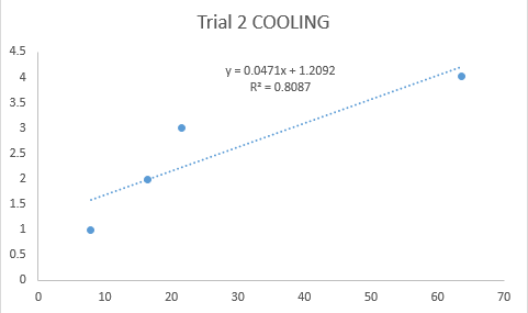
Figure 3. Plot of the Linearization of Equation 1 for Cooling Procedure
Figure 4 below shows the one of the plots for the heating procedure.
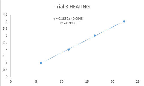
Figure 4. Plot of the Linearization of Equation 1 for Heating Procedure
The thermal time constant, t’, can be calculated by getting the reciprocal of the slope of the plotted graphs. The average thermal time constant obtained from the heating procedure was 4.67. For the cooling procedure, the average thermal time constant was 27.3. The obtained thermal time constants should have been the same, but due to a lot of factors we could not control such as the temperature change as the thermometer was transferred, or the heat from our hands.
